
Theme: Clinical Resarch
In this page, I’d like to present how to analyze clinical data in various statistical ways
Dataset One : Measure of Exposure to Lead-based materials
Exposure to lead can produce a variety of adverse health effects in infants and children, including hyperactivity, hearing or memory loss, learning disabilities, and damage to the nervous system.
Much of the exposure to lead is due to deteriorating lead-based paint that may be chipping and peeling in older homes. Lead-based paint in housing was banned in the US in 1978; however, many older homes (built pre-1978) do contain lead-based paint, and chips and dust can be ingested by young children living in these homes during normal teething and hand-to-mouth behavior. The US Center for Disease Control and Prevention has conducted a study on the efficacy of a treatment succimer that helps remove the lead that has been ingested by a child. In a clinic, 120 children aged 12–36 months were randomly allocated into three groups, labeled 1, 2, and 3, respectively: 40 children were assigned to receive a placebo, 40 a low dose of succimer, and 40 a high dose of succimer. Patients were to return to the clinic at weeks 2, 4, 6, and 8. At each visit, whether feeling sick (fever, fuzziness, etc.) and blood lead level were measured for each child. Also, gender and age at the baseline (in months) were recorded.
Data preparation: Creating into a Long-form, Normality Check
Source Code in R Language


Normality Check
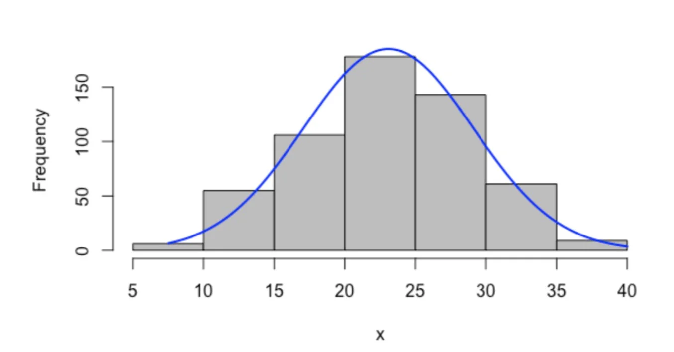
With p-value greater than 0.05
The measure of lead is
normally distributed.
Therefore, I can go further analysis.

The above step is done with hypothesis testing.
Individual profiles plot: Variation Check

The individual profiles plot shows enough variation such that the analysis can go further.
Since the dataset is measured repeated times on a single individual and the response variable (lead) has distribution with enough variation, fitting on a random intercept linear regression model is required.
Results After fitting the regression model
Used languages: R, SAS


The fitted model equation

In order to use the equation, just plug in the test subject’s profile in corresponding types; numeric and categorical.
Prediction example

The predicted result of lead level for a such patient/ individual is
18.5719
Interpretation of the fitted regression model estimates
As the size of group increases by one person, the estimated average blood lead level decreases by 0.93 points.
As age increases by one month, the estimated average blood lead level increases by 0.26 points.
As week increases by one week, the estimated average blood lead level decreases by 1.006454 points.
Another Way to build a prediction model is
Nonparametric regression; loess function
Fitting the loess function Source Code in R

Plotting the fitted regression model


The prediction result from the loess regression is
20.01841
Data description
Dataset Two: Seizures
With controlled experiment

Client
Name here
Year
01/01/000
Client
Name here
Year
01/01/000
The data in the file “seizures_data.csv” are from a clinical trial conducted on 40
subjects suffering from epileptic seizures who were randomized to receive a
placebo (20 subjects) or the anti-seizure agent progabide (20 subjects). Whether
the subjects experienced a seizure between two consecutive visits was recorded
during each of four post-treatment two-week periods. The baseline variables are
age, gender, and the number of diagnosed common epilepsy comorbid
conditions: bone deterioration and fractures, stroke, depression, migraine, and
attention-deficit hyperactivity disorder.
The response variable is Binary
The model used:
Binary regression model with a random intercept.
Source Code (SAS and R, respectively)


Output with Estimated Coefficients and test statistics
-
![]()
SAS output
-
![]()
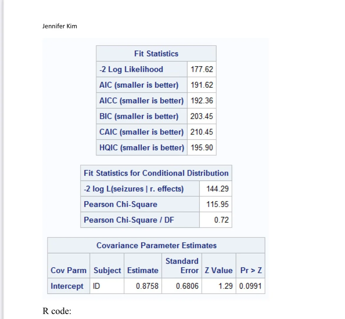
SAS output with Test statistic
-
![]()
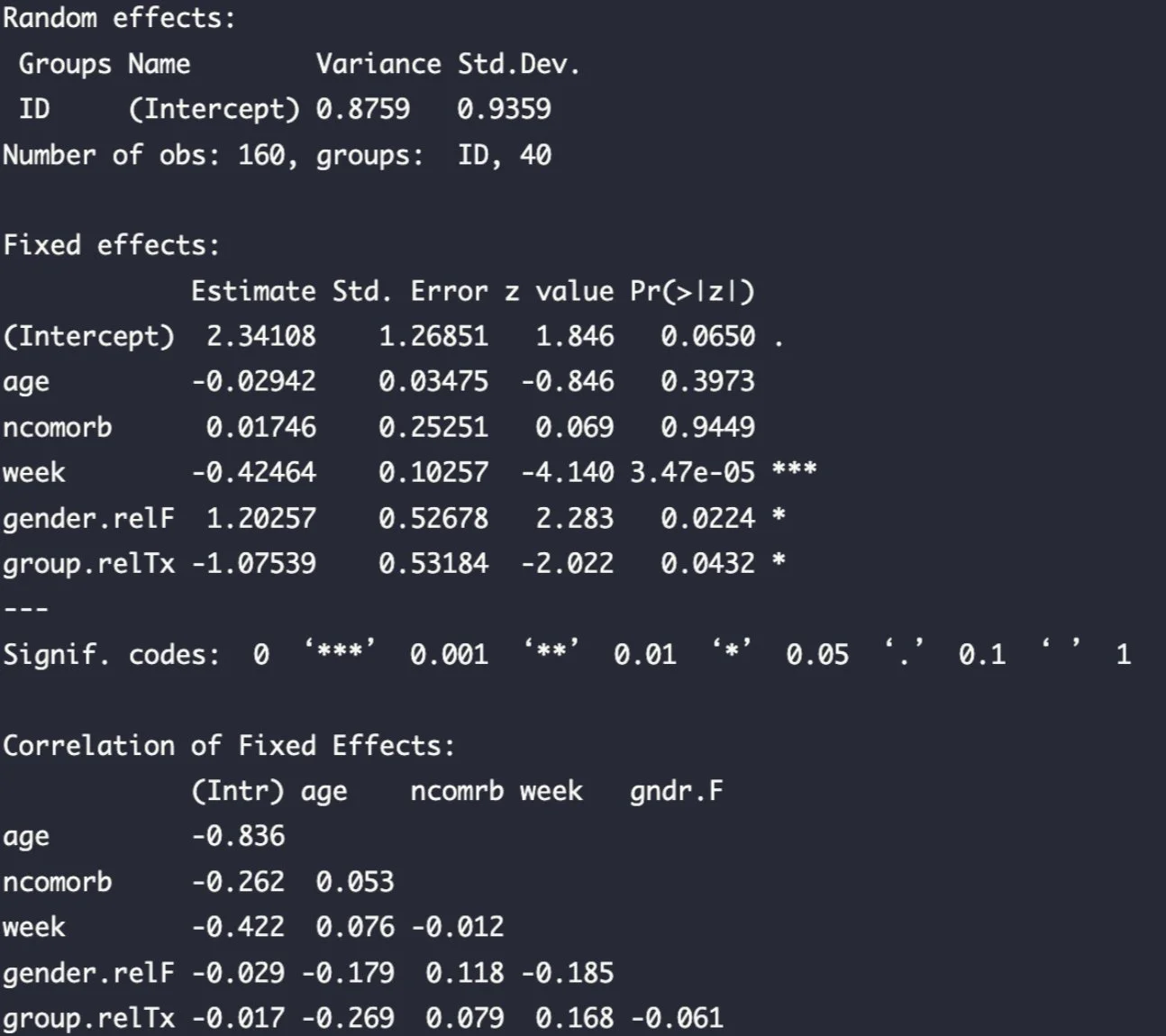
R output
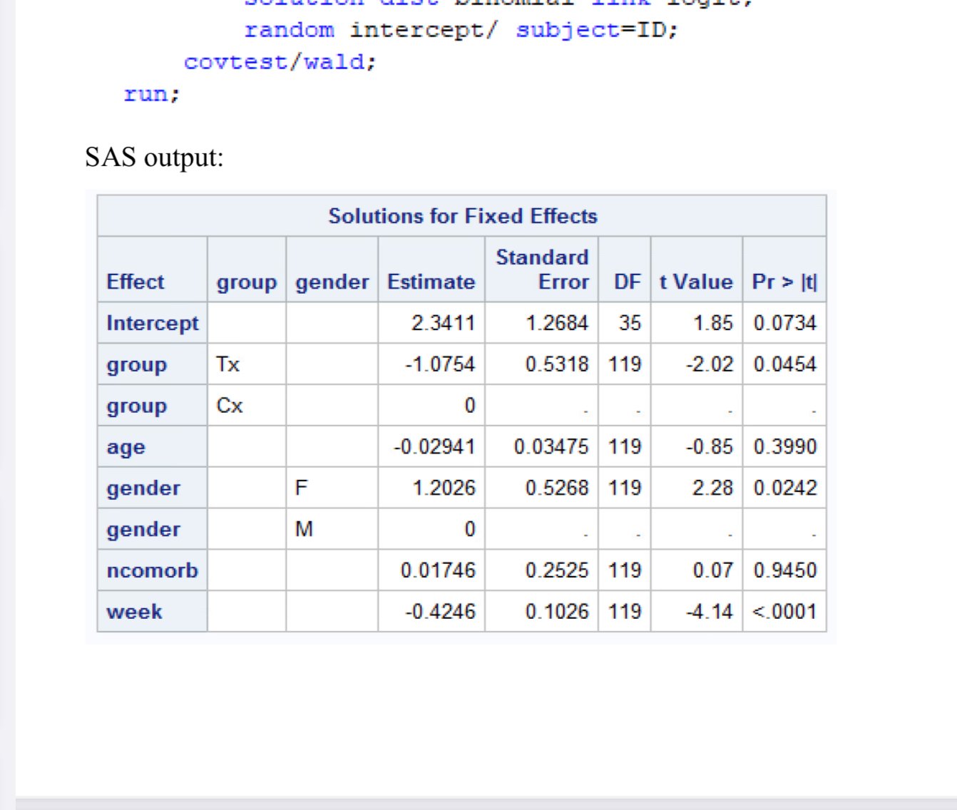
Interpretation

Prediction Profile
ID#: 41
Group placed in: Control group
Age : 35
Gender : Female
Number of comorbidities: 3
Week: 6th / 8th
Prediction


Prediction Results


The hand calculation has been double checked. The reason it differs from the results from the two softwares can vary.